CubeSolver - Solving Algorithms
There are many methods to solve the Rubik's Cube. They have different characteristics and are dedicated to different uses:
- Some are easy to learn.
- Some allow solving the cube quickly.
- Some are applicable to multiple cube sizes.
- Some allow solving the cube in few moves.
Two methods are currently implemented in CubeSolver:
- The Jessica Fridrich method, implemented with evolutionary population-based solution searching.
- The Thistlethwaite method.
After presenting how these two algorithms work, their performance will be studied and compared.
Evolutionary Algorithm / Exhaustive OLL and PLL Search
The method applied is Jessica Fridrich's method. The only difference is that the corners of the first layer and the edges of the second layer are solved in two steps, not one. (No F2L for those familiar with it).
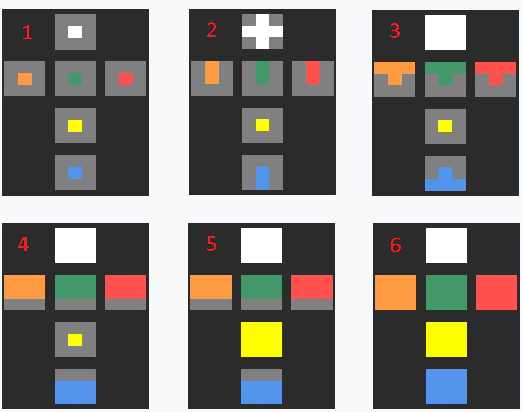
The different steps are:
- Any scrambled cube
- A cube with the white cross solved
- A cube with the first layer solved
- A cube with the first two layers solved
- A cube with the first two layers solved, and the pieces of the last layer correctly oriented
- A solved cube
The first two layers are solved using an evolutionary algorithm, the last layer is solved by exhaustive search through a series of sequences.
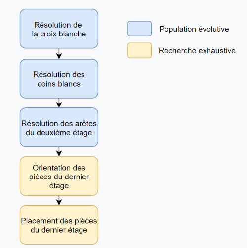
Solving the First Two Layers by Evolutionary Population
This is the first solving algorithm I implemented, inspired by a genetic algorithm without actually being one.
As a reminder, here is the schematic summary of how a genetic algorithm works:
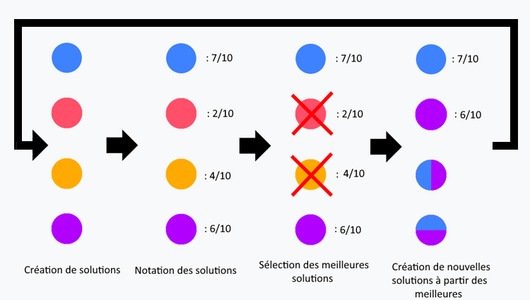
The main choices related to developing such an algorithm concern:
- Creating a heuristic to score each solution.
- The number of "individuals" to keep at each iteration.
- How new solutions can be created from old ones.
Why Not Directly Apply a Genetic Algorithm?
It is difficult to apply such an algorithm to solving a Rubik's Cube because of the last step, also called "cross-over".
To create a new individual from two parents, you need to mix the "genes" of these two parents. These genes can be of different natures depending on the problem (such as numbers that can be averaged), but in our case, remember that each solution is a sequence of movements.
Here, the movements that make up these solutions only make sense within their sequence.
If the sequence 1 – 2 – 3 – 4 is promising, And the sequence 9 – 8 – 7 – 6 too, I have no guarantee that the sequence 1 – 8 – 3 – 6 or even 1 – 2 – 7 – 6 is interesting.
Thus, applying a cross-over to solutions, and therefore "mixing" two parents, seems difficult. Instead, it's possible to add random elements to the end of an interesting sequence.
For example, if the sequence 1 – 2 – 3 – 4 has good results, we can try the sequence 1 – 2 – 3 – 4 – 9.
We thus "repopulate" our set of solutions by adding random elements to previously selected solutions.
That's how this algorithm works. The implementation is available here.
Each iteration is broken down into three steps:
- Score each individual in our population.
- Select the best individuals.
- Recreate a population from the survivors. And the algorithm stops when an individual achieves the goal.
The heuristic (the method of scoring individuals) depends on the stages of the solve. The goal is to reward individuals approaching the solution; we can therefore give points to a sequence when certain pieces are at certain positions.
We have three parameters for our algorithm:
- What is the size of our population?
- How many individuals do we select at each iteration?
- When creating new individuals, how many movements do we add?
Solving the Last Layer by Exhaustive Search
The number of possible sequences to orient and permute the pieces of the last layer is very small (57 for orientation and 21 for permutation). Thus, testing all these sequences (hard-coded in the code) guarantees solving the last layer quickly and simply.
This method comes directly from Jessica Fridrich's method; the use of these 78 sequences is classic in the speedcubing world. They are therefore named: OLL (Orientation of Last Layer) and PLL (Permutation of Last Layer). You can find all the information about them here and here. The implementation is available here.
Thistlethwaite's Algorithm
Morwen Thistlethwaite is a British mathematician who developed a famous solution for the Rubik's Cube. This algorithm consists of several steps, each of which involves bringing the cube into a position where it can be solved using a subset of moves. Thus, at each step, the number of possible configurations of the cube decreases, until reaching the final state.
This article is illustrated with a solving example. Here is the cube that will be solved:
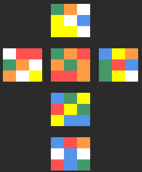
And here is the scramble associated with this cube: [D, F', R2, B2, R, U', D2, F2, L2, U', F2, L, D', L, B', F', R, D']
First Step:
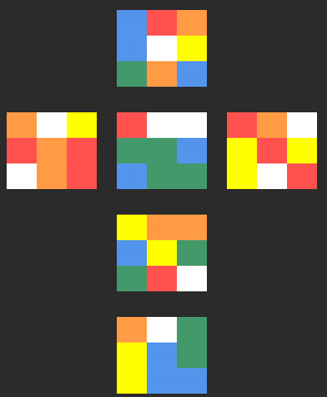
- Solution:
[B, R', D', L', U'] - Goal: Orient the twelve edges of the Rubik's cube.
- Search space:
<L, R, F, B, U, D> - Search space reduction: We stop using quarter turns of the U (Up) and D (Down) faces.
Indeed, an edge is said to be correctly oriented if it is possible to solve it without using quarter turns of the top and bottom faces. Once all edges are correctly oriented, it is possible to solve the cube without using these two movements, so we can ignore them.
Second Step:
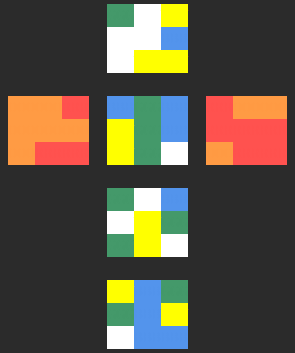
- Solution:
[B', D2, R', F', L', F', R', B'] - Goal: Orient the eight corners of the Rubik's cube, and group all M-slice edges into the M slice.
- Search space:
<L, R, F, B, U2, D2> - Search space reduction: We stop using quarter turns of the F (Front) and B (Back) faces.
A corner is said to be correctly oriented if its L / R color is present on its L / R face. Once we stop using quarter turns of the F / B faces, it will be impossible to modify the orientation of the corners, which will therefore remain in their correct orientation until the end of the solve. The M slice is the one between the L / R faces. Similarly, once the M edges are placed in the M slice, they can no longer leave it since we'll stop using quarter turns of the F / B faces.
Third Step:
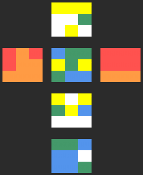
- Solution:
[R2, B2, R, D2, R'] - Goal: Bring each corner into its "natural orbit".
- Search space:
<L, R, F2, B2, U2, D2> - Search space reduction: /
A corner is said to be "placed in its natural orbit" if it can be solved using only double moves (L2, R2, F2, B2, U2, D2). There are only 96 corner positions meeting this requirement.
Fourth Step:
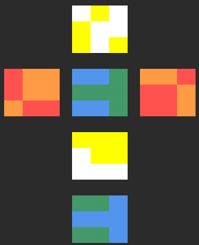
- Solution:
[B2, R', B2, D2, B2, U2, D2, L'] - Goal: Bring each edge into its final slice.
- Search space:
<L, R, F2, B2, U2, D2> - Search space reduction: We stop using quarter turns of the L / R faces.
Once the edges of each slice (M, E, and S) are brought into their final slice, they can thus be solved using only double moves.
Fifth Step:

- Solution:
[R2, U2, R2, U2, R2, F2, D2, F2, R2, B2, D2] - Goal: Solve the Rubik's cube.
- Search space:
<L2, R2, F2, B2, U2, D2>
The cube can now be solved using only double turns, and a solution can be found relatively quickly.
Implementation
My implementation of this algorithm is available here.
The solution search algorithm used is IDDFS (Iterative Deepening Depth First Search). It is a derivative of DFS, traversing solutions in an order similar to BFS.
Algorithm Performance
Defining Performance
Algorithm performance can be defined by two criteria:
- The average solving speed of a cube.
- The average number of moves needed for a solve.
The Importance of Implementation
The execution speed of an algorithm depends greatly on the quality of its implementation. To achieve the best possible performance, the critical parts of the code and the data architecture must be optimized. To perform this optimization, we can use a CPU Profiler. This tool allows real-time determination of which parts of our code consume the most resources. The developer's work is thus greatly facilitated, as they can focus their attention on the important elements.
Algorithm Performance
We can observe that Thistlethwaite's algorithm takes much longer to execute, but produces much shorter sequences. All values presented below are averages over 100 solves.
Thistlethwaite's Algorithm:
- Average solving time: 253.35 seconds (4 minutes 13 seconds)
- Average number of moves: 36.23 moves
Evolutionary Algorithm:
-
Population size: 100
-
Surviving population percentage: 10
-
Number of random mutations: between 1 and 5
-
Average solving time: 0.36 seconds
-
Average number of moves: 101
A more detailed examination of performance will be available in a future version of the site.